Algorithms

Algorithms put the science in computer science.

Permutation

If we have n items, we can order them in n factorial ( n! ) different ways.

Permutation with Identical items

The factorial n! overcounts the number of ways to order n items if some are identical. Identical items swapping their positions shouldn’t count as a different permutation.

In a sequence of n items of which r are identical, there are r! ways to reorder identical items. Thus, n! counts each distinct per- mutation r! times. To get the number of distinct permutations, we need to divide n! by this overcount factor.

For instance, the number of distinct permutations of the letters “ CODE ENERGY ” is 10!/3!

Combinations

Picture a deck of 13 cards containing all spades. How many ways can you deal six cards to your opponent? We’ve seen 13!/(13 − 6)! is the number of permutations of six out of 13 possible items. Since the order of the six cards doesn’t matter, we must divide this by 6! to obtain:

13!/6!(13-60)!

a permutation is an ordered combination

Sum

Calculating sums of sequences occurs often when counting. Sequen- tial sums are expressed using the capital-sigma ( Σ ) notation.

4
∑ (2i + 1) = 1 + 3 + 5 + 7 + 9.
i=0

Example 1

You need to fly to New York City anytime in the next 30 days.
Air ticket prices change unpredictably according to the departure 
and  return dates.How many pairs of days must be checked to find 
the cheapest tickets for flying to NYC and back within the next 30 days?

Solution

Hence, 30 pairs begin with day 1, 29 pairs begin with
day 2, 28 with day 3, and so on. 
There’s only one pair that begins on day 30.
So 30+29+...+2+1 is the total number of pairs ∑ 30

30
∑ i = 30(30 + 1)/2 = 465 pairs
i=1

Example 2

1,2,3,4,5
how many 3 digit odd numbers can be formed?

Solution

4way x 3way x 1 = 12
4way x 3way x 3 = 12
4way x 3way x 5 = 12

sum 36 ways

Strategy

Handle repetitive tasks through iteration , Iterate elegantly using recursion , Use brute force when you’re lazy but powerful, Test bad options and then backtrack , Save time with heuristics for a reasonable way out, Divide and conquer your toughest opponents, Identify old issues dynamically not to waste energy again, Bound your problem so the solution doesn’t escape.

The iterative strategy consists in using loops (e.g. for , while ) to repeat a process until a condition is met. Each step in a loop is called an iteration .

the power set (or powerset) of any set S is the set of all subsets of S, including the empty set and S itself,

Brute Force

The brute force strategy solves problems by inspecting all of the problem’s possible solution candidates.

Backtracking

sudoku solve method

Heuristics

A heuristic method , or simply a heuristic , is a method that leads to a solution without guaranteeing it is the best or optimal one. Heuristics can help when methods like brute force or backtracking are too slow.

Greedy Algorithms

Greedy algorithms try to find a localized optimum solution, which may eventually lead to globally optimized solutions. However, generally greedy algorithms do not provide globally optimized solutions.

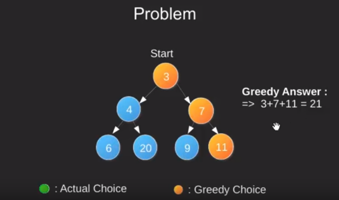
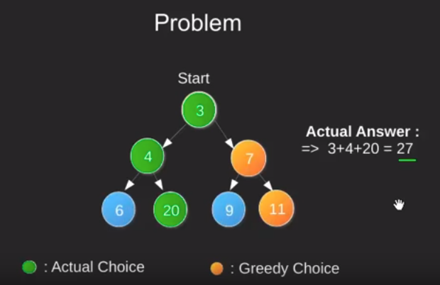
Most networking algorithms use the greedy approach. Here is a list of few of them

• Travelling Salesman Problem
• Prim’s Minimal Spanning Tree Algorithm
• Kruskal’s Minimal Spanning Tree Algorithm
• Dijkstra’s Minimal Spanning Tree Algorithm
• Graph - Map Coloring
• Graph - Vertex Cover
• Knapsack Problem
• Job Scheduling Problem

Divide and Conquer (D&C)

To recap, here’s how D&C works:

1. Figure out a simple case as the base case.
2. Figure out how to reduce your problem and get to the base case.

Example:

Suppose you’re a farmer with a plot of land. 1680x640 meters
You want to divide this farm evenly into square plots. 
You want the plots to be as big as possible. 

1. Figure out the base case. This should be the simplest possible case. When the recursive function will end to call itself.
2. Divide or decrease your problem until it becomes the base case.

Suppose one side is 25 meters (m) and the other side is 50 m. Then the largest box you can use is 25 m × 25 m. You need two of those boxes to divide up the land.

Now you need to figure out the recursive case. This is where D&C comes in. According to D&C, with every recursive call, you have to reduce your problem. How do you reduce the problem here? Let’s start by marking out the biggest boxes you can use.

So you started out with a 1680 × 640 farm that needed to be split up. But now you need to split up a smaller segment, 640 × 400. If you find the biggest box that will work for this size, that will be the biggest box that will work for the entire farm. You just reduced the problem from a 1680 × 640 farm to a 640 × 400 farm

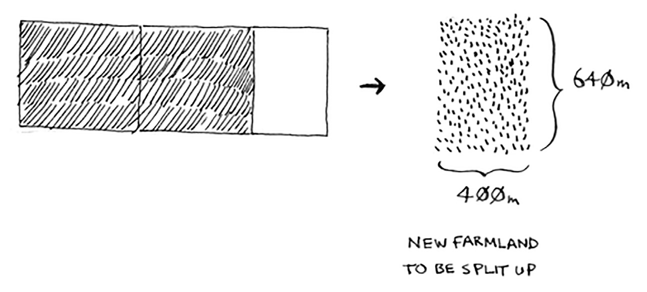
you draw a box on that to get an even smaller segment. at the end the biggest plot size you can use is 80 × 80 m

This is Euclid’s algorithm

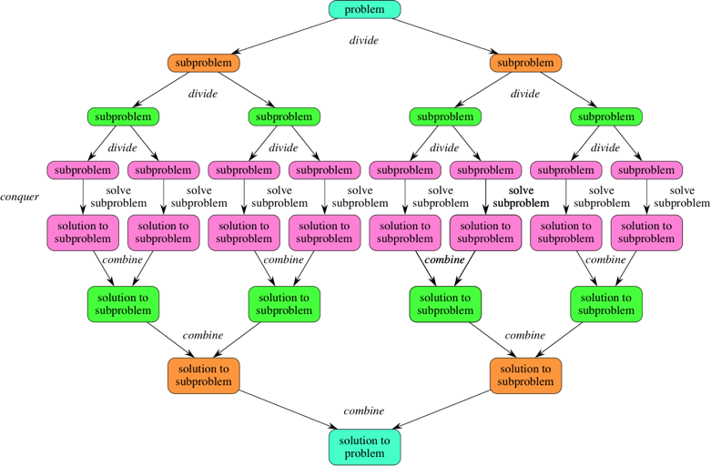
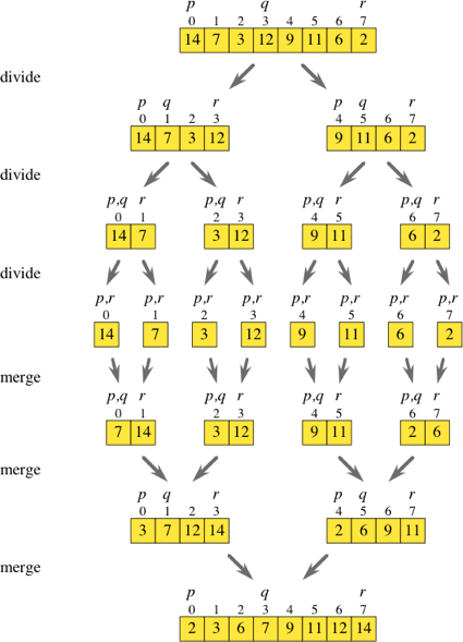
1. Divide the problem into a number of subproblems that are smaller instances of the same problem.
2. Conquer the subproblems by solving them recursively. If they are small enough, solve the subproblems as base cases.
3. Combine the solutions to the subproblems into the solution for the original problem.

Dynamic Programming

Dynamic programming starts by solving subproblems and builds up to solving the big problem. Dynamic programming approach is similar to divide and conquer in breaking down the problem into smaller and yet smaller possible sub-problems.

Dynamic programming is used where we have problems, which can be divided into similar sub-problems, so that their results can be reused. Mostly, these algorithms are used for optimization. Before solving the inhand subproblem, dynamic algorithm will try to examine the results of the previously solved subproblems. The solutions of subproblems are combined in order to achieve the best solution.

It can be hard to come up with a dynamic-programming solution. That’s what we’ll focus on in this section. Some general tips follow:

• Every dynamic-programming solution involves a grid.
• The values in the cells are usually what you’re trying to optimize. For the knapsack problem, the values were the value of the goods.
• Each cell is a subproblem, so think about how you can divide your problem into subproblems. That will help you figure out what

The following computer problems can be solved using dynamic programming approach

• Fibonacci number series
• Knapsack problem
• Tower of Hanoi
• All pair shortest path by Floyd-Warshall
• Shortest path by Dijkstra
• Project scheduling

Dynamic programming can be used in both top-down and bottom-up manner.

Branch and Bound

Algorithm Complexity

Analysis of algorithm is the process of analyzing the problem-solving capability of the algorithm in terms of the time and size required.

• Time Factor − Time is measured by counting the number of key operations such as comparisons in the sorting algorithm.
• Space Factor − Space is measured by counting the maximum memory space required by the algorithm.

Algorithm falls under three types

• Best Case − Minimum time required for program execution.
• Average Case − Average time required for program execution.
• Worst Case − Maximum time required for program execution.
• Amortized − A sequence of operations applied to the input of size a averaged over time.

BigO - how time scales with respect to some input variables

Computational Complexity

• P - problems solvable in polynamial time
• EXP - problems solvable in exponential time
• R - problems solvable in finite time

n - input 
k - loop 

P - n , nxn
P - (n^k) 
EXP - (k^n)

NP = solvable in P on a nondeterministic machine

P ≠ NP hard to solve easy to verify(examples: riddles, puzzle without picture,secret key encryption)

O(n+c) = O(n)
O(cn) = O(n), c>0

f(n) = 7log(n)^3 + 15n^2 + 2n^3 + 8
O(f(n)) = O(n^3)

Common Asymptotic Notations

n size of the input

Constant:	O(1)
Logarithmic:	O(log(n))
Linear:		O(n)
Linearithmic:	O(nlog(n))
Quadtic:	O(n^2)
Cubic:		O(n^3)
Polynomial:	nΟ(1)
Exponential:	O(b^n)b>1
Factorial:	O(n!)

Constant Time

O(1)

a = 1
b = 2
c = a+5*b

i = 0
while i < 11
	i = i+1;

Linear Time

O(n)

i = 0
while i < n 
	i = i+1

// f(n) = n
// O((f(n))) = O(n)	

i=0
while i<n 
	i=i+3
// f(n) = n/3
// O((f(n))) = O(n)

Quadtic Time

O(n^2)

for(i = 0, i < n , i++) {
	for(j=0;j<n;j++) { // }
}

// f(n) = n*n = n^2
// O(f(n)) = O(n^2)

for(i=0;i<n;i++)
	for(j=i;j < n;j++)

Divide and Conquer (D&C)

To recap, here’s how D&C works:

1. Figure out a simple case as the base case.
2. Figure out how to reduce your problem and get to the base case.

Example:

Suppose you’re a farmer with a plot of land. 1680x640 meters

You want to divide this farm evenly into square plots. You want the plots to be as big as possible.

1. Figure out the base case. This should be the simplest possible case. When the recursive function will end to call itself.

2. Divide or decrease your problem until it becomes the base case.

Suppose one side is 25 meters (m) and the other side is 50 m. Then the largest box you can use is 25 m × 25 m. You need two of those boxes to divide up the land.

Euclid’s algorithm

Sneak peak at functional programming

Inductive proofs

1. Divide the problem into a number of subproblems that are smaller instances of the same problem.
2. Conquer the subproblems by solving them recursively. If they are small enough, solve the subproblems as base cases.
3. Combine the solutions to the subproblems into the solution for the original problem.

Divide-and-conquer

The following computer algorithms are based on divide-and-conquer programming approach −

Merge Sort Quick Sort Binary Search Strassen’s Matrix Multiplication Closest pair (points)

Average case vs. worst case

Categories of algorithms

Search − Algorithm to search an item in a data structure. Sort − Algorithm to sort items in a certain order. Insert − Algorithm to insert item in a data structure. Update − Algorithm to update an existing item in a data structure. Delete − Algorithm to delete an existing item from a data structure.

Algorithm Complexity

Time Factor − Time is measured by counting the number of key operations such as comparisons in the sorting algorithm. Space Factor − Space is measured by counting the maximum memory space required by the algorithm.

Algorithm falls under three types

Best Case − Minimum time required for program execution. Average Case − Average time required for program execution. Worst Case − Maximum time required for program execution.

Common Asymptotic Notations

constant − Ο(1) logarithmic − Ο(log n) linear − Ο(n) n log n − Ο(n log n) quadratic − Ο(n2) cubic − Ο(n3) polynomial − nΟ(1) exponential − 2Ο(n)

Greedy Algorithms

Greedy algorithms try to find a localized optimum solution, which may eventually lead to globally optimized solutions. However, generally greedy algorithms do not provide globally optimized solutions.

Most networking algorithms use the greedy approach. Here is a list of few of them −

Travelling Salesman Problem Prim’s Minimal Spanning Tree Algorithm Kruskal’s Minimal Spanning Tree Algorithm Dijkstra’s Minimal Spanning Tree Algorithm Graph - Map Coloring Graph - Vertex Cover Knapsack Problem Job Scheduling Problem

The Knapsack problem

The set-covering problem

Combinatorics

Approximation algorithms

Dynamic Programming

Dynamic programming starts by solving subproblems and builds up to solving the big problem.

• Dynamic programming is useful when you’re trying to optimize something given a constraint. In the knapsack problem, you had to maximize the value of the goods you stole, constrained by the size of the knapsack. • You can use dynamic programming when the problem can be broken into discrete subproblems, and they don’t depend on each other.

It can be hard to come up with a dynamic-programming solution. That’s what we’ll focus on in this section. Some general tips follow:

• Every dynamic-programming solution involves a grid. • The values in the cells are usually what you’re trying to optimize. For the knapsack problem, the values were the value of the goods. • Each cell is a subproblem, so think about how you can divide your problem into subproblems. That will help you figure out what the axes are.

The Feynman algorithm

Longest common subsequence

Longest common substring

Levenshtein distance

k-nearest neighbors

Pythagorean formula

Cosine similarity

• KNN is used for classification and regression and involves looking at the k-nearest neighbors. • Classification = categorization into a group. • Regression = predicting a response (like a number).

Dynamic Programming

Dynamic programming approach is similar to divide and conquer in breaking down the problem into smaller and yet smaller possible sub-problems.

Dynamic programming is used where we have problems, which can be divided into similar sub-problems, so that their results can be re-used. Mostly, these algorithms are used for optimization. Before solving the in-hand sub-problem, dynamic algorithm will try to examine the results of the previously solved sub-problems. The solutions of sub-problems are combined in order to achieve the best solution.

The following computer problems can be solved using dynamic programming approach −

Fibonacci number series Knapsack problem Tower of Hanoi All pair shortest path by Floyd-Warshall Shortest path by Dijkstra Project scheduling

Dynamic programming can be used in both top-down and bottom-up manner.