Data Structure
28 March 2018 · Filed in TutorialAbstract Data Type
An Abstract Data Type (ADT) is the specification of a group of operations that make sense for a given data type.
Primitive data types
Primitive data types are those with built-in support in the programming language you’re using—they work without external modules. These always include integers, floating points, 3 and generic operations with them (addition, subtraction, division).
Structures
An Abstract Data Type only describes how variables of a given data type are operated. It provides a list of operations, but doesn’t explain how data operations happen. Conversely, data structures describe how data is to be organized and accessed in the computer’s memory. They provide ways for implementing ADTs in data-handling modules.
Abstract Data Types
| Abstract Data Type | Other Common Names | Commonly Implemented With |
|---|---|---|
| List | Sequence | Array,Linked List |
| Queue | Array,Linked List | |
| Double Ended Queue | Equeue, Deque | Array,Doubly Linked List |
| Stack | Array,Linked List | |
| Associative Array | Dictionary, Hash Map, Hash, Map | Hash Table |
| Set | Red-Black Tree,Hash Table | |
| Priority Queue | Heap | Heap |
Container List Set Multiset Map Multimap Graph Stack Queue Priority queue Double-ended queue Double-ended priority queue
Linear Data Structures
Hash-Based Data Structures
Trees
Binary Search Trees
Heaps
Graphs
Strings
Lists
A list is an abstract data type used for storing sequential items
The head is the first item in the list.
The tail is all remaining items.
The tail is itself a list, having its own head and tail:
| Function | Functionality |
|---|---|
| new | Creates an empty list. |
| append | Adds an item to the end of the list. |
| prepend | Adds an item to the beginning of the list. |
| head | Returns the item at the beginning of the list. |
| tail | Returns all items except the head. If the list only has 1 item, returns an empty list. |
| is_empty | Returns a bool indicating whether or not the list contains any items. |
Stack
Stack can be implemented with a variety of data structures, such as a linked list or an array
LIFO data structure. LIFO stands for Last-in-first-out.
| Function | Functionality |
|---|---|
| push(i) | Insert element i at the top of the stack. |
| pop() | Remove the element at the top of the stack. |
| peek() | returns the element at the top of the stack without changing the stack |
| size() | returns the current size of the stack |
| isFull() | check if stack is full. |
| isEmpty() | check if stack is empty. |
Time Complexity
| Function | Linked list | Array |
|---|---|---|
| push() | O(1) | O(1) |
| pop() | O(1) | O(1) |
Queue
Queue is an abstract data structure, somewhat similar to Stacks. Unlike stacks, a queue is open at both its ends. One end is always used to insert data (enqueue) and the other is used to remove data (dequeue). Queue follows First-In-First-Out methodology, i.e., the data item stored first will be accessed first.
| Function | Functionality |
|---|---|
| enqueue(i) | Insert element i at the tail of the queue. |
| dequeue() | Remove the element at the head of the queue. |
| peek() | returns the element at the head of the queue without changing the queue. |
| size() | returns the current size of the queue |
| isfull() | Checks if the queue is full. |
| isempty() | Checks if the queue is empty. |
Time Complexity
| Function | Linked list | Array |
|---|---|---|
| enqueue() | O(1) | O(n) |
| dequeue() | O(1) | O(n) |
Double Ended Queues
Double ended queues, called deques for short, are a generalized form of the queue. It is exactly like a queue except that elements can be added to or removed from the head or the tail
| Function | Functionality |
|---|---|
| append(i) | Adds element i to the tail of the queue |
| prepend(i) | Adds element i to the head of the queue |
| delete_last() | Removes the element at the tail of the queue |
| delete_first() | Removes the element at the head of the queue |
| examine_last() | Returns the element at the tail of the queue |
| examine_first() | Returns the element at the head of the queue |
Time Complexity
| Operation | Doubly Linked List | Dynamic Array |
|---|---|---|
| append | O(1) | O(1) |
| prepend | O(1) | O(n) |
| delete_last | O(1) | O(1) |
| delete_first | O(1) | O(n) |
| examine_last | O(1) | O(1) |
| examine_first | O(1) | O(1) |
Priority Queue
Priority queues are a kind of abstract data type that generalizes the queue. Their principles are exactly the same except that they also include a priority for every value in the queue. When a value is inserted, a priority is assigned to it. The value with the highest priority is always removed first.
| Function | Functionality |
|---|---|
| insert(i, p) | Add value i with priority p. |
| pop() | Remove and return the element with the highest priority. |
| peek() | Return the element with the highest priority without changing the queue. |
Time Complexity
| Function | Heap |
|---|---|
| insert(i, p) | O(logn) |
| pop() | O(logn) |
| peek() | O(1) |
Sets
Sets are a type of abstract data type that allows you to store a list of non-repated values. Their name derives from the mathematical concept of finite sets. Unlike an array, sets are unordered and unindexed These are the two properties of a set: the data is unordered and it is not duplicated.
| Function | Functionality |
|---|---|
| insert(i) | Adds i to the set |
| remove(i) | Removes i from the set |
| size() | Returns the size of the set |
| contains(i) | Returns whether or not the set contains i |
| union(S, T) | Returns the union of set S and set T |
| intersection(S, T) | Returns the intersection of set S and set T |
| difference(S, T) | Returns the difference of set S and set T |
| subset(S, T) | Returns whether or not set S is a subset of set T |
Time Complexity
A hash table is the most common data structure
| Function | Hash table |
|---|---|
| insert() | O(1) |
| contains() | O(1) |
| remove() | O(1) |
Array
The array is a basic abstract data type that holds an ordered collection of items accessible by an integer index. These items can be anything from primitive types such as integers to more complex types like instances of classes. Since it’s an ADT, it doesn’t specify an implementation, but is almost always implemented by an array (data structure) or dynamic array. They are extremely ubiquitous and among the oldest, most widely used data structures in programming.
Unless otherwise specified, for the remainder of this wiki, the word “array” will refer to the data structure and not the abstract data type.
Arrays are often used to implement abstract data types such as arrays (ADT) and stacks.
In Java, you can create an array of any primitive data type, abstract data type, or custom class. Java also provides an ArrayList type which gives you more flexibility.
Following are the basic operations supported by an array.
- Traverse − print all the array elements one by one.
- Insertion − Adds an element at the given index.
- Deletion − Deletes an element at the given index.
- Search − Searches an element using the given index or by the value.
- Update − Updates an element at the given index.
| Operation | Array | ArrayList | Linked List |
|---|---|---|---|
| Read | O(1) | O(1) | O(n) |
| Add/Remove at end | O(1) | O(1) | O(n) |
| Add/Remove in the interior | O(n) | O(n) | O(n) |
| Resize | O(n) | N/A | N/A |
| Find By position | O(1) | O(1) | O(n) |
| Find By value | O(n) | O(n) | O(n) |
Dynamic arrays
Dynamic arrays are the next logical extension of arrays.
Associative Array
Associative arrays, also called maps or dictionaries, are an abstract data type that can hold data in (key, value) pairs.
| Function | Functionality |
|---|---|
| insert(key, value) | Add a (key, value) pair to the associative array |
| remove(key) | Remove the key’s pair in the associative array |
| update(key, value) | Assigns/updates the value to/of the existing key |
| lookup(key) | Returns the value assigned to this key |
Time Complexity
| Function | Array | Red-Black Tree | Hash Table |
|---|---|---|---|
| insert | O(n) | O(log(n)) | O(1) |
| remove | O(n) | O(log(n)) | O(1) |
| update | O(n) | O(log(n)) | O(1) |
| lookup | O(n) | O(log(n)) | O(1) |
Linked list
Types of Linked List
- Simple Linked List − Item navigation is forward only.
- Doubly Linked List − Items can be navigated forward and backward.
- Circular Linked List − Last item contains link of the first element as next and the first element has a link to the last element as previous.
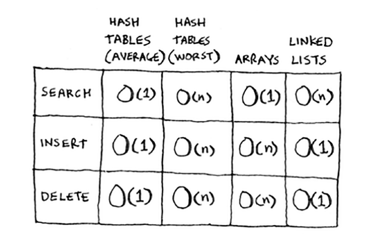
Hash tables
They’re also known as hash maps, maps, dictionaries,and associative arrays.
Python has hash tables; they’re called dictionaries.
>>> phone_book = {}
Same as phone_book = dict()
Binary Search Tree
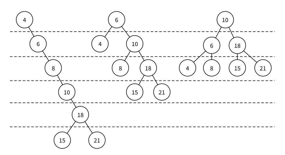
A Binary Search Tree is a special type of Tree that can be efficiently searched. Nodes in Binary Search Trees can have at most two chil- dren. And nodes are positioned according to their value/key. Children nodes to the left of the parent must be smaller than the parent, children nodes to the right must be greater.
Tree Balancing
If we insert too many nodes in a Binary Search Tree, we end up with a tree of very high height, where many nodes have only one child. But we can rearrange nodes in a tree such that its height is reduced. This is called tree balancing . A perfectly balanced tree has the minimum possible height.
The Red-Black Tree
The Red-Black Tree is a famous example of a self-balancing tree, which colors nodes either “red” or “black” for its balancing strat- egy.
The AVL Tree
The AVL Tree is another breed of self-balancing trees. They require a bit more time to insert and delete items than Red-Black Trees, but tend to have better balancing. This means they’re faster than Red-Black Trees for retrieving items. AVL Trees are often used to optimize performance in read-intensive scenarios.
The Binary Heap
The Binary Heap is a special type of Binary Search Tree, in which we can find the smallest (or highest) item instantly. This data structure is especially useful for implementing Priority Queues. In the Heap it costs O(1) to get the minimum (or maximum) item, be- cause it is always the Root Node of the tree. Searching or inserting nodes still costs O( log n) . It has the same node placement rules as the Binary Search Tree, plus an extra restriction: a parent node must be greater (or smaller) than both its child nodes.

The Graph
The Graph is similar to the Tree. The difference is that there’s no children or parent nodes, and therefore, no Root Node. For example, graphs are ideal for representing a social network, where nodes are people and edges represent friendships.
Types of Graphs
- Undirected Graph - A undirected graph contains edges but the edges are not directed ones.
- Directed Graph - In a directed graph, each edge has a direction.
- Weighted Graphs - edges has weight to represent an value
Rerpresenting Graphs
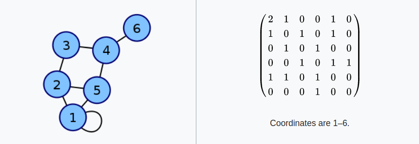
an adjacency matrix is a square matrix used to represent a finite graph. The elements of the matrix indicate whether pairs of vertices are adjacent or not in the graph.
Tree
A tree in an undirectect graph with no cycles.
Breadth-first search
The algorithm to solve a shortest-path problem is called breadth-first search.
Each graph is made up of nodes and edges. (A) —edge—> (B) A and B are neighbors
• Question type 1: Is there a path from node A to node B? • Question type 2: What is the shortest path from node A to node B?
Graphs
Graph Implementations
Edge lists
| One simple way to represent a graph is just a list, or array, of | E | ∣E∣vertical bar, E, vertical bar edges, which we call an edge list. To represent an edge, we just have an array of two vertex numbers, or an array of objects containing the vertex numbers of the vertices that the edges are incident on |
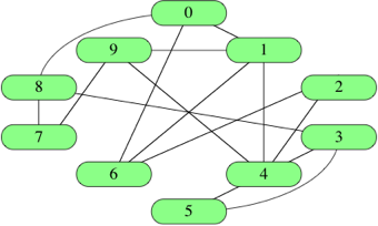
[ [0,1], [0,6], [0,8], [1,4], [1,6], [1,9], [2,4], [2,6], [3,4], [3,5],
[3,8], [4,5], [4,9], [7,8], [7,9] ]
Adjacency Matrix
| For a graph with | V | ∣V∣vertical bar, V, vertical bar vertices, an adjacency matrix is a | V | \times | V | ∣V∣×∣V∣vertical bar, V, vertical bar, times, vertical bar, V, vertical bar matrix of 0s and 1s, where the entry in row i ii and column j jj is 1 if and only if the edge (i,j) (i,j)left parenthesis, i, comma, j, right parenthesis is in the graph. |
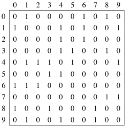
Directed Graph Unweighted graph boolean Weighted graph values
Adjacency List
| Representing a graph with adjacency lists combines adjacency matrices with edge lists. For each vertex i ii, store an array of the vertices adjacent to it. We typically have an array of | V | ∣V∣vertical bar, V, vertical bar adjacency lists, one adjacency list per vertex. |
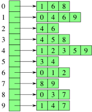
In JavaScript, we represent these adjacency lists by:
[ [1, 6, 8],
  [0, 4, 6, 9],
  [4, 6],
  [4, 5, 8],
  [1, 2, 3, 5, 9],
  [3, 4],
  [0, 1, 2],
  [8, 9],
  [0, 3, 7],
  [1, 4, 7] ]
Graph Traversals
Depth First Search (DFS)
Depth First Search (DFS) algorithm traverses a graph in a depthward motion and uses a stack to remember to get the next vertex to start a search, when a dead end occurs in any iteration.
Rule 1 − Visit the adjacent unvisited vertex. Mark it as visited. Display it. Push it in a stack. Rule 2 − If no adjacent vertex is found, pop up a vertex from the stack. (It will pop up all the vertices from the , which do not have adjacent vertices.) Rule 3 − Repeat Rule 1 and Rule 2 until the stack is empty.
Breadth First Search (BFS)
Breadth First Search (BFS) algorithm traverses a graph in a breadthward motion and uses a queue to remember to get the next vertex to start a search, when a dead end occurs in any iteration.
Rule 1 − Visit the adjacent unvisited vertex. Mark it as visited. Display it. Insert it in a queue. Rule 2 − If no adjacent vertex is found, remove the first vertex from the queue. Rule 3 − Repeat Rule 1 and Rule 2 until the queue is empty.
Dijkstra’s algorithm
Tree
Tree represents the nodes connected by edges.
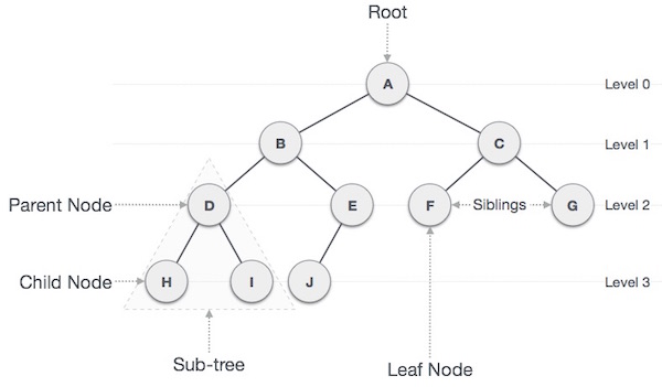
every tree have n nodes n-1 edges
Binary Search Tree
A Binary Search Tree (BST) is a tree in which all the nodes follow the below-mentioned properties −
The left sub-tree of a node has a key less than or equal to its parent node’s key.
The right sub-tree of a node has a key greater than to its parent node’s key.
https://www.youtube.com/playlist?list=PLDV1Zeh2NRsDGO4–qE8yH72HFL1Km93P
References
- https://www.geeksforgeeks.org/top-algorithms-and-data-structures-for-competitive-programming/
- https://www.tutorialspoint.com/data_structures_algorithms
- https://brilliant.org/practice/abstract-data-types-intro/?subtopic=types-and-data-structures
- http://bigocheatsheet.com/
